Cdf of Continuous Uniform Distribution Over the Unit Circle

Uniform distribution on an interval

Uniform
Probability density function 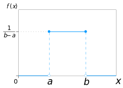Using maximum convention
Cumulative distribution function
Notation	${\mathcal {U}}_{[a,b]}$
Parameters	$-\infty <a<b<\infty \,$
Support	$x\in [a,b]$
PDF	${\begin{cases}{\frac {1}{b-a}}&{\text{for }}x\in [a,b]\\0&{\text{otherwise}}\end{cases}}$
CDF	${\begin{cases}0&{\text{for }}x<a\\{\frac {x-a}{b-a}}&{\text{for }}x\in [a,b]\\1&{\text{for }}x>b\end{cases}}$
Mean	${\tfrac {1}{2}}(a+b)$
Median	${\tfrac {1}{2}}(a+b)$
Mode	any value in $(a,b)$
Variance	${\tfrac {1}{12}}(b-a)^{2}$
MAD	${\tfrac {1}{4}}(a+b)$
Skewness	0
Ex. kurtosis	$-{\tfrac {6}{5}}$
Entropy	$\ln(b-a)\,$
MGF	${\begin{cases}{\frac {\mathrm {e} ^{tb}-\mathrm {e} ^{ta}}{t(b-a)}}&{\text{for }}t\neq 0\\1&{\text{for }}t=0\end{cases}}$
CF	${\begin{cases}{\frac {\mathrm {e} ^{itb}-\mathrm {e} ^{ita}}{it(b-a)}}&{\text{for }}t\neq 0\\1&{\text{for }}t=0\end{cases}}$

In probability theory and statistics, the continuous uniform distribution or rectangular distribution is a family of symmetric probability distributions. The distribution describes an experiment where there is an arbitrary outcome that lies between certain bounds.^[1] The bounds are defined by the parameters, a and b, which are the minimum and maximum values. The interval can either be closed (e.g. [a, b]) or open (e.g. (a, b)).^[2] Therefore, the distribution is often abbreviated U (a, b), where U stands for uniform distribution.^[1] The difference between the bounds defines the interval length; all intervals of the same length on the distribution's support are equally probable. It is the maximum entropy probability distribution for a random variable X under no constraint other than that it is contained in the distribution's support.^[3]

Definitions [edit]

Probability density function [edit]

The probability density function of the continuous uniform distribution is:

f(x)={\begin{cases}{\frac {1}{b-a}}&\mathrm {for} \ a\leq x\leq b,\\[8pt]0&\mathrm {for} \ x<a\ \mathrm {or} \ x>b\end{cases}}

The values of f(x) at the two boundaries a and b are usually unimportant because they do not alter the values of the integrals of $f (x) dx$ over any interval, nor of $x f (x) dx$ or any higher moment. Sometimes they are chosen to be zero, and sometimes chosen to be $1 / b - a$ . The latter is appropriate in the context of estimation by the method of maximum likelihood. In the context of Fourier analysis, one may take the value of f(a) or f(b) to be $1 / 2(b - a)$ , since then the inverse transform of many integral transforms of this uniform function will yield back the function itself, rather than a function which is equal "almost everywhere", i.e. except on a set of points with zero measure. Also, it is consistent with the sign function which has no such ambiguity.

Graphically, the probability density function is portrayed as a rectangle where $b-a$ is the base and $\scriptstyle {\frac {1}{b-a}}$ is the height. As the distance between a and b increases, the density at any particular value within the distribution boundaries decreases.^[4] Since the probability density function integrates to 1, the height of the probability density function decreases as the base length increases.^[4]

In terms of mean μ and variance σ ², the probability density may be written as:

f(x)={\begin{cases}{\frac {1}{2\sigma {\sqrt {3}}}}&{\mbox{for }}-\sigma {\sqrt {3}}\leq x-\mu \leq \sigma {\sqrt {3}}\\0&{\text{otherwise}}\end{cases}}

Cumulative distribution function [edit]

The cumulative distribution function is:

F(x)={\begin{cases}0&{\text{for }}x<a\\[8pt]{\frac {x-a}{b-a}}&{\text{for }}a\leq x\leq b\\[8pt]1&{\text{for }}x>b\end{cases}}

Its inverse is:

F^{-1}(p)=a+p(b-a)\,\,{\text{ for }}0<p<1

In mean and variance notation, the cumulative distribution function is:

F(x)={\begin{cases}0&{\text{for }}x-\mu <-\sigma {\sqrt {3}}\\{\frac {1}{2}}\left({\frac {x-\mu }{\sigma {\sqrt {3}}}}+1\right)&{\text{for }}-\sigma {\sqrt {3}}\leq x-\mu <\sigma {\sqrt {3}}\\1&{\text{for }}x-\mu \geq \sigma {\sqrt {3}}\end{cases}}

and the inverse is:

F^{-1}(p)=\sigma {\sqrt {3}}(2p-1)+\mu \,\,{\text{ for }}0\leq p\leq 1

Example 1. Using the Uniform Cumulative Distribution Function [edit]

For random variable $X$

X\sim U(0,23)

Find $\scriptstyle P(2<X<18)$ :

P(2<X<18)=(18-2)\cdot {\frac {1}{23-0}}={\frac {16}{23}}

In graphical representation of uniform distribution function [f(x) vs x], the area under the curve within the specified bounds displays the probability (shaded area is depicted as a rectangle). For this specific example above, the base would be $\scriptstyle 18-2$ and the height would be $\scriptstyle {\frac {1}{23}}$ .^[5]

Example 2. Using the Uniform Cumulative Distribution Function (Conditional) [edit]

For random variable $X$

X\sim U(0,23)

Find $\scriptstyle P(X>12\ |\ X>8)$ :

P(X>12\ |\ X>8)=(23-12)\cdot {\frac {1}{23-8}}={\frac {11}{15}}

The example above is for a conditional probability case for the uniform distribution: given $\scriptstyle X>8$ is true, what is the probability that $\scriptstyle X>12$ . Conditional probability changes the sample space so a new interval length $b-a$ has to be calculated, where $b$ is 23 and $a$ is 8.^[5] The graphical representation would still follow Example 1, where the area under the curve within the specified bounds displays the probability and the base of the rectangle would be $\scriptstyle 23-12$ and the height $\scriptstyle {\frac {1}{15}}$ .^[5]

Generating functions [edit]

Moment-generating function [edit]

The moment-generating function is:^[6]

M_{x}=E(e^{tx})={\frac {e^{tb}-e^{ta}}{t(b-a)}}\,\!

^[7]

from which we may calculate the raw moments m _k

m_{1}={\frac {a+b}{2}},\,\!

m_{2}={\frac {a^{2}+ab+b^{2}}{3}},\,\!

m_{k}={\frac {1}{k+1}}\sum _{i=0}^{k}a^{i}b^{k-i}.\,\!

For the special case a = –b, that is, for

f(x)={\begin{cases}{\frac {1}{2b}}&{\text{for}}\ -b\leq x\leq b,\\[8pt]0&{\text{otherwise}},\end{cases}}

the moment-generating functions reduces to the simple form

M_{x}={\frac {\sinh bt}{bt}}.

For a random variable following this distribution, the expected value is then m ₁ = (a +b)/2 and the variance is m ₂ −m ₁ ² = (b −a)²/12.

Cumulant-generating function [edit]

For $n \geq 2$ , the nth cumulant of the uniform distribution on the interval $[-1/2, 1/2]$ is B _n/n, where B _n is the nth Bernoulli number.^[8]

Standard uniform [edit]

Restricting $a=0$ and $b=1$ , the resulting distribution U(0,1) is called a standard uniform distribution.

One interesting property of the standard uniform distribution is that if u ₁ has a standard uniform distribution, then so does 1-u ₁. This property can be used for generating antithetic variates, among other things. In other words, this property is known as the inversion method where the continuous standard uniform distribution can be used to generate random numbers for any other continuous distribution.^[4] If $u$ is a uniform random number with standard uniform distribution (0,1), then $x=F^{-1}(u)$ generates a random number $x$ from any continuous distribution with the specified cumulative distribution function $F$ .^[4]

Relationship to other functions [edit]

As long as the same conventions are followed at the transition points, the probability density function may also be expressed in terms of the Heaviside step function:

f(x)={\frac {\operatorname {H} (x-a)-\operatorname {H} (x-b)}{b-a}},\,\!

or in terms of the rectangle function

f(x)={\frac {1}{b-a}}\,\operatorname {rect} \left({\frac {x-\left({\frac {a+b}{2}}\right)}{b-a}}\right).

There is no ambiguity at the transition point of the sign function. Using the half-maximum convention at the transition points, the uniform distribution may be expressed in terms of the sign function as:

f(x)={\frac {\operatorname {sgn} {(x-a)}-\operatorname {sgn} {(x-b)}}{2(b-a)}}.

Properties [edit]

Moments [edit]

The mean (first moment) of the distribution is:

E(X)={\frac {1}{2}}(b+a).

The second moment of the distribution is:

E(X^{2})={\frac {b^{3}-a^{3}}{3b-3a}}.

In general, the n-th moment of the uniform distribution is:

E(X^{n})={\frac {b^{n+1}-a^{n+1}}{(n+1)(b-a)}}

The variance (second central moment) is:

V(X)={\frac {1}{12}}(b-a)^{2}

Order statistics [edit]

Let X ₁, ..., X _n be an i.i.d. sample from U(0,1). Let X _(k) be the kth order statistic from this sample. Then the probability distribution of X _(k) is a Beta distribution with parameters k and n − k + 1. The expected value is

\operatorname {E} (X_{(k)})={k \over n+1}.

This fact is useful when making Q–Q plots.

The variances are

\operatorname {V} (X_{(k)})={k(n-k+1) \over (n+1)^{2}(n+2)}.

See also: Order statistic § Probability distributions of order statistics

Uniformity [edit]

The probability that a uniformly distributed random variable falls within any interval of fixed length is independent of the location of the interval itself (but it is dependent on the interval size), so long as the interval is contained in the distribution's support.

To see this, if X ~ U(a,b) and [x, x+d] is a subinterval of [a,b] with fixed d > 0, then

P\left(X\in \left[x,x+d\right]\right)=\int _{x}^{x+d}{\frac {\mathrm {d} y}{b-a}}\,={\frac {d}{b-a}}\,\!

which is independent of x. This fact motivates the distribution's name.

Generalization to Borel sets [edit]

This distribution can be generalized to more complicated sets than intervals. If S is a Borel set of positive, finite measure, the uniform probability distribution on S can be specified by defining the pdf to be zero outside S and constantly equal to 1/K on S, where K is the Lebesgue measure of S.

[edit]

If X has a standard uniform distribution, then by the inverse transform sampling method, Y = − λ⁻¹ ln(X) has an exponential distribution with (rate) parameter λ.
If X has a standard uniform distribution, then Y = X ⁿ has a beta distribution with parameters (1/n,1). As such,
The standard uniform distribution is a special case of the beta distribution with parameters (1,1).
The Irwin–Hall distribution is the sum of n i.i.d. U(0,1) distributions.
The sum of two independent, equally distributed, uniform distributions yields a symmetric triangular distribution.
The distance between two i.i.d. uniform random variables also has a triangular distribution, although not symmetric.

Statistical inference [edit]

Estimation of parameters [edit]

Estimation of maximum [edit]

Minimum-variance unbiased estimator [edit]

Given a uniform distribution on [0,b] with unknown b, the minimum-variance unbiased estimator (UMVUE) for the maximum is given by

{\hat {b}}_{\text{UMVU}}={\frac {k+1}{k}}m=m+{\frac {m}{k}}

where m is the sample maximum and k is the sample size, sampling without replacement (though this distinction almost surely makes no difference for a continuous distribution). This follows for the same reasons as estimation for the discrete distribution, and can be seen as a very simple case of maximum spacing estimation. This problem is commonly known as the German tank problem, due to application of maximum estimation to estimates of German tank production during World War II.

Maximum likelihood estimator [edit]

The maximum likelihood estimator is given by:

{\hat {b}}_{ML}=m

where m is the sample maximum, also denoted as $m=X_{(n)}$ the maximum order statistic of the sample.

Method of moment estimator [edit]

The method of moments estimator is given by:

{\hat {b}}_{MM}=2{\bar {X}}

where ${\bar {X}}$ is the sample mean.

Estimation of midpoint [edit]

The midpoint of the distribution (a +b) / 2 is both the mean and the median of the uniform distribution. Although both the sample mean and the sample median are unbiased estimators of the midpoint, neither is as efficient as the sample mid-range, i.e. the arithmetic mean of the sample maximum and the sample minimum, which is the UMVU estimator of the midpoint (and also the maximum likelihood estimate).

Confidence interval [edit]

For the maximum [edit]

Let X ₁, X ₂, X ₃, ..., X _n be a sample from $U_{[0,L]}$ where L is the population maximum. Then X _(n) = max( X ₁, X ₂, X ₃, ..., X _n ) has the Lebesgue-Borel-density $f:={\frac {d\Pr _{X_{(n)}}}{d\lambda }}$ ^[9]

f(t)=n{\frac {1}{L}}\left({\frac {t}{L}}\right)^{n-1}=n{\frac {t^{n-1}}{L^{n}}},0\leq t\leq L

The confidence interval given before is mathematically incorrect, as $\Pr([{\hat {\theta }},{\hat {\theta }}+\epsilon ]\ni \theta )\geq 1-\alpha$ cannot be solved for $\epsilon$ without knowledge of $\theta$ . However one can solve

\Pr([{\hat {\theta }},{\hat {\theta }}(1+\epsilon )]\ni \theta )\geq 1-\alpha

for

\epsilon \geq (1-\alpha )^{-1/n}-1

for any unknown but valid

\theta

one then chooses the smallest $\epsilon$ possible satisfying the condition above. Note that the interval length depends upon the random variable ${\hat {\theta }}$ .

Occurrence and applications [edit]

The probabilities for uniform distribution function are simple to calculate due to the simplicity of the function form.^[2] Therefore, there are various applications that this distribution can be used for as shown below: hypothesis testing situations, random sampling cases, finance, etc. Furthermore, generally, experiments of physical origin follow a uniform distribution (e.g. emission of radioactive particles).^[1] However, it is important to note that in any application, there is the unchanging assumption that the probability of falling in an interval of fixed length is constant.^[2]

Economics example for uniform distribution [edit]

In the field of economics, usually demand and replenishment may not follow the expected normal distribution. As a result, other distribution models are used to better predict probabilities and trends such as Bernoulli process.^[10] But according to Wanke (2008), in the particular case of investigating lead-time for inventory management at the beginning of the life cycle when a completely new product is being analyzed, the uniform distribution proves to be more useful.^[10] In this situation, other distribution may not be viable since there is no existing data on the new product or that the demand history is unavailable so there isn't really an appropriate or known distribution.^[10] The uniform distribution would be ideal in this situation since the random variable of lead-time (related to demand) is unknown for the new product but the results are likely to range between a plausible range of two values.^[10] The lead-time would thus represent the random variable. From the uniform distribution model, other factors related to lead-time were able to be calculated such as cycle service level and shortage per cycle. It was also noted that the uniform distribution was also used due to the simplicity of the calculations.^[10]

Sampling from an arbitrary distribution [edit]

The uniform distribution is useful for sampling from arbitrary distributions. A general method is the inverse transform sampling method, which uses the cumulative distribution function (CDF) of the target random variable. This method is very useful in theoretical work. Since simulations using this method require inverting the CDF of the target variable, alternative methods have been devised for the cases where the CDF is not known in closed form. One such method is rejection sampling.

The normal distribution is an important example where the inverse transform method is not efficient. However, there is an exact method, the Box–Muller transformation, which uses the inverse transform to convert two independent uniform random variables into two independent normally distributed random variables.

Quantization error [edit]

In analog-to-digital conversion a quantization error occurs. This error is either due to rounding or truncation. When the original signal is much larger than one least significant bit (LSB), the quantization error is not significantly correlated with the signal, and has an approximately uniform distribution. The RMS error therefore follows from the variance of this distribution.

Random variate generation [edit]

There are many applications in which it is useful to run simulation experiments. Many programming languages come with implementations to generate pseudo-random numbers which are effectively distributed according to the standard uniform distribution. On the other hand, the uniformly distributed numbers are often used as the basis for non-uniform random variate generation.

If u is a value sampled from the standard uniform distribution, then the value a + (b − a)u follows the uniform distribution parametrised by a and b, as described above.

History [edit]

While the historical origins in the conception of uniform distribution are inconclusive, it is speculated that the term 'uniform' arose from the concept of equiprobability in dice games (note that the dice games would have discrete and not continuous uniform sample space). Equiprobability was mentioned in Gerolamo Cardano's Liber de Ludo Aleae, a manual written in 16th century and detailed on advanced probability calculus in relation to dice.^[11]

References [edit]

^ ^a ^b ^c Dekking, Michel (2005). A modern introduction to probability and statistics : understanding why and how . London, UK: Springer. pp. 60–61. ISBN978-1-85233-896-1.
^ ^a ^b ^c Walpole, Ronald; et al. (2012). Probability & Statistics for Engineers and Scientists. Boston, USA: Prentice Hall. pp. 171–172. ISBN978-0-321-62911-1.
^ Park, Sung Y.; Bera, Anil K. (2009). "Maximum entropy autoregressive conditional heteroskedasticity model". Journal of Econometrics. 150 (2): 219–230. CiteSeerX10.1.1.511.9750. doi:10.1016/j.jeconom.2008.12.014.
^ ^a ^b ^c ^d "Uniform Distribution (Continuous)". MathWorks. 2019. Retrieved November 22, 2019.
^ ^a ^b ^c Illowsky, Barbara; et al. (2013). Introductory Statistics. Rice University, Houston, Texas, USA: OpenStax College. pp. 296–304. ISBN978-1-938168-20-8.
^ Casella & Berger 2001, p. 626
^ https://www.stat.washington.edu/~nehemyl/files/UW_MATH-STAT395_moment-functions.pdf^{[ bare URL PDF ]}
^ https://galton.uchicago.edu/~wichura/Stat304/Handouts/L18.cumulants.pdf^{[ bare URL PDF ]}
^ Nechval KN, Nechval NA, Vasermanis EK, Makeev VY (2002) Constructing shortest-length confidence intervals. Transport and Telecommunication 3 (1) 95-103
^ ^a ^b ^c ^d ^e Wanke, Peter (2008). "The uniform distribution as a first practical approach to new product inventory management". International Journal of Production Economics. 114 (2): 811–819. doi:10.1016/j.ijpe.2008.04.004 – via Research Gate.
^ Bellhouse, David (May 2005). "Decoding Cardano's Liber de Ludo". Historia Mathematica. 32: 180–202. doi:10.1016/j.hm.2004.04.001.

External links [edit]

Online calculator of Uniform distribution (continuous)

woodstren2002.blogspot.com

Source: https://en.wikipedia.org/wiki/Continuous_uniform_distribution